Oblique and cross-grid UAV imaging flight plans – a sneak preview of the analysis of resulting 3D point cloud properties for deciduous forest surfaces – low cost 3D mapping with the Phantom 4R (RTK)

Flight plans / photogrammetry / structure from motion / Metashape / oblique imaging / 3D point clouds / Lastools / Phantom 4R RTK / beech tree / deciduous trees / forest stand structure

“Oblique and cross-grid UAV imaging flight plans – a sneak preview of the analysis of resulting 3D point cloud properties for deciduous forest surfaces” by Sören Hese.

Various flight plan configuration options exist for UAV based photogrammetric data acquisitions with SfM approaches. Especially for discontinuous surfaces the imaging configurations can make a difference for the resulting point cloud density and 3D properties of the point cloud. This work tries to quantify the differences for a deciduous beech and oak tree dominated forest with data captured with a Phantom 4 RTK in different setups.

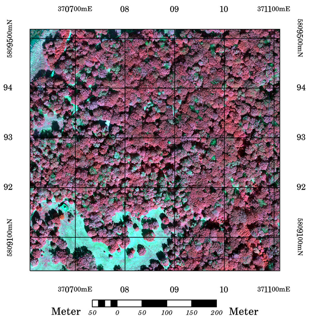
The test site is situated within the historical landscape park area “Klein Glienicke” in the south-west of Berlin. This area belongs to the UNESCO world heritage sites of Berlin/Brandenburg.

The leaf-on flights were performed in 78 m altitude with 85/85 percent image overlap using 60 degrees oblique viewing angles for oblique imaging. The leaf-off flight was performed in 120m altitude. Direct sunlight light illumination situation with data captured between 11AM and 1PM CEST. Overcast conditions were captured June 29th for comparison. Processing was done using keypoint and tiepoint limit set to “off” and full resolution processing with 20 MP image files, no point cloud (depth) filtering. Full processing parameters are listed in table 1.

P4RTK Flight & Processing Parameters	Leaf-On flight 3.6.2022 direct sunlight	Leaf-On flight 29.6.2022 overcast	Leaf-Off flight 31.3.2021 direct sunlight
Align quality	high (full resolution images)	high	high
Keypoint limit	0 (off)	0 (off)	80 000
Tiepoint limit	0 (off)	0 (off)	10 000
Dense point quality	full res. (20 MP)	full res. (20 MP)	full res. (20 MP)
Dense point cloud depth filtering	no depth filtering	no depth filtering	no depth filtering
Projection	WGS84 UTM33N	WGS84 UTM33N	WGS84 UTM33N
Build DSM (digital surface model)	hole filling=no	hole filling=no	hole filling=no
No. of images	N:334, DGN:649, O2:508, O4:1020, O4N:1268, O4DGN:1669.	N:240, DGN:651, O2:500, O4:1018, O4N:1266, O4DGN:1669.	O4N: 1055
Flight altitude (pixel res.)	78 m (2 cm)	78 m (2 cm)	120 m (2.5 cm)
Image overlap	85/85	85/85	85/85
Viewing angle (degree)	90 Nadir/60 oblique	90 Nadir/60 oblique	90 Nadir/60 oblique
No. points in models (millions)	578, 752, 728, 1006, 1101, 1281	456, 787, 739, 1063, 1165, 1253	472

The following flight plans were investigated:

• Nadir flight tracks (85/85) (N) 90 degree Nadir viewing only – standard flight mode,
• Double Grid Nadir flight tracks (85/85)(DGN), 90 degree Nadir viewing (cross grid mode),
• Oblique 2 directions – double grid oblique (85/85)(O2), 60 degree oblique viewing (cross grid with 2 viewing directions),
• Oblique 4 directions – forward and backward viewing with two double grids (NWSE viewing) (85/85) (O4) , 60 degree oblique viewing (viewing in 4 directions),
• Oblique 4 directions (NWSE viewing) with additional one Nadir flight track (85/85) )O4N), 60 degree oblique viewing and 90 degree Nadir, (same as O4 but with additional N),
• Oblique 4 directions (NWSE viewing) with additional Double Grid Nadir flight tracks (85/85) (O4DGN), 60 degree oblique viewing and 90 degree Nadir viewing (combination of DGN and O4).

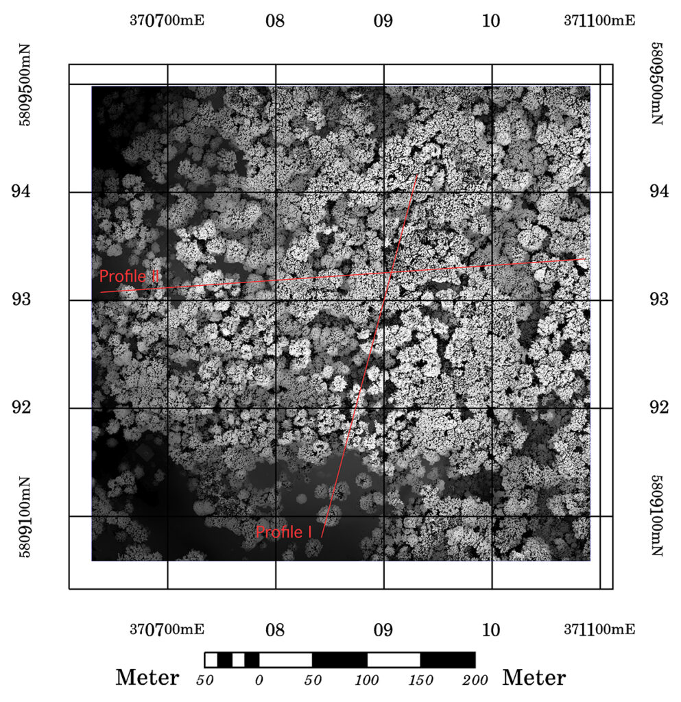
The resulting P4RTK geo-positioned jpegs were directly processed in Metashape 1.8.3 in full resolution mode (alignment quality “high”, dense point cloud “ultra high” setting) with no tiepoint or keypoint limitations. The derived dense point clouds were processed without depth filtering, projected to WGS84 UTM33N and sliced into two transects – each 1 m wide using lastools: las2las -keep_profile. One transect goes from south to north through the forested region, the other from east to west. Within the transects the ground height points were classified to id=2 using lasground_new and the number of ground points was calculated for all flight plans and transects. The transects were also directly visualized with lasview.

The different flight plans lead to point clouds with different densities in the 1 m wide profiles:

Flight plan type	| No. of points in profile I (NS) (ground points)	| No. of points in profile II (EW) (ground points)
N	898 891 (91 295)	1 128 998 (26 961)
DGN	1 232 924 (89 188)	1 483 073 (35 850)
O2	1 310 647 (92 780)	1 717 351 (60 585)
O4	1 737 963 (107 699)	2 319 041 (74 480)
O4N	1 889 683 (113 294)	2 507 219 (62 256)
O4DGN	2 213 784 (123 077)	2 809 812 (78 421)

The following lastools processing steps were performed to generate the CHM point cloud and starting analysis on the CHM point cloud:

Cutting the full point cloud into a subset for the multiview angle analysis were full overlap of all images in guaranteed. This is easily done with lasclip.

lasclip -i lasfile.laz -poly mvsubarea.shp -o out.laz

Cutting the subarea point cloud into slices for profile analysis (and later into tiles) and for further CHM processing (the full model is to big for TIN based CHM processing in lasground_new:

las2las -i input.laz -keep_profile 371056.154 5809332.601 370646.508 5809307.474 8 -o out.laz

Filtering: we filtered the extreme point cloud outliers for further processing to CHM heights. This is kind of difficult since we only want to remove clear outlier – within the dense point cloud these outlier usually come in clusters so removing these needs some specific settings especially with the “-isolated” value. In this dataset the isolated clusters have a lot of points but they are far away from the main terrain surface and canopy volume. Grid boxes of size 1x1x1 m are only point cleared when neighbouring boxes all have less than “-isolated”. This is clearly a powerful parameter and here the higher this value the stronger the filtering but it might leave some noise close to the below terrain heigh level. Reducing the step value by 50% (box grid size) with interactive control was a strategy that was successful but might not be easily transferrable to other point cloud datasets and you have to readjust the “-isolated value here also by factor .25 since its volumen and not side length.

lasnoise -i file.laz -v -remove_noise -isolated 300 -step_xy 1 -step_z 1 -o outfiltered.laz

lasnoise -i file.laz -v -remove_noise -isolated 80 -step_xy 0.5 -step_z 0.5 -o outfiltered.laz

Canopy Height Model calculation on profiles: finally deriving the CHM profiles was done using lasground_new with testing the -hyper_fine / -fine / – coarse settings and using -all_returns and without. Here we directly write the new difference height into the new z value field and generate the CHM point cloud. The important control parameters in lasground_new are “-step”, “-offset” and “-refine”. The -spike options are usable to filter out some noise here but I prefer to remove noise in lasnoise. Obviously the naming convention of input output files is kind of crucial to not get totally confused when this is done for the various flight modi transects.

lasground_new -i file.laz -fine -all_returns -step 25 -compute_height -replace_z -o CHM.laz

lasground_new -i tiles/o4n/*.laz -hyper_fine -v -ignore_first_of_many -ignore_intermediate -step 10 -offset 0.09 -odir tiles\o4n-g -olaz -cores 20 // to directly convert to chm: -step 25 -compute_height -replace_z -o CHM.laz

lasinfo -i classified-groundfile.laz -o groundfile.lasinfo.txt

Quantitative comparison of the point clouds can be done nicely with lasinfo, lascanopy and lasvoxel. Lasinfo writes a summary of the laz file (min/max/no point/point density/various attributes) into a text file. lascanopy is creating a lot of different canopy metrics based on polygons or grid descriptions, and lasvoxel does a voxelization with a defined square size and counting of intensities – however lasvoxel writes a laz file. The resulting lazfile can be used to store the number of points per voxel with the -step-z-infinite parameter. This saves the number of returns for all vertical voxels in one grid cell to the intensity value.

lasvoxel -i input.laz -step-z-infinite step_xy 0.5 -o VOXEL-InfZ-out.laz

The intensity is now useful to compare the number of point returns in one voxel column. This is done by gridding the voxel laz file to a tif file. In order to save the intensity as grey value this is done with the -intensity value:

las2dem -i VOXEL-InfZ-out.laz -o DEM-VOXEL-InfZ-out.tif -intensity

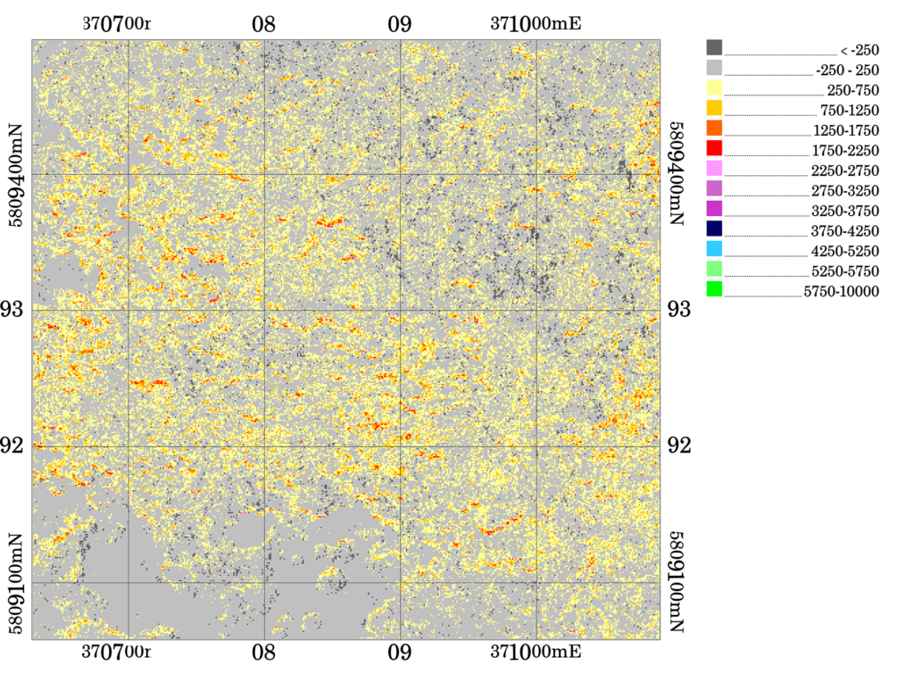
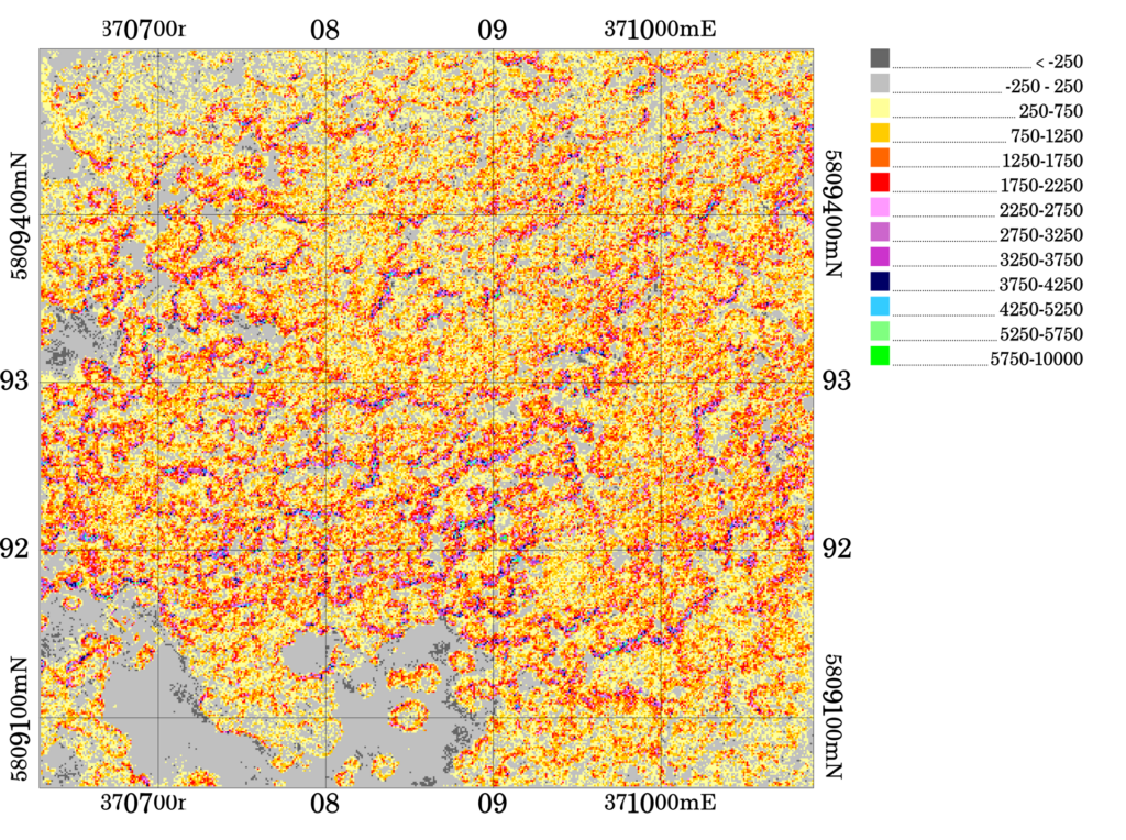
Comparison of point densities can now be done easily with the raster tif formats. For this work difference raster files were created with the simple Nadir flight modi (N) as the reference showing spatially where the point density is changed most between the different flight plan modi (Fig. 4 and Fig. 5).

For the full CHM point cloud calculation the original point clouds were subsetted to the study region, then filtered for outlier and indexed. Indexing is useful to speed up the tiling process. Tiling was then done to 100×100 m tiles to ease the lasground_new process. Both processes can be accelerated on multiple las input files/tiles with -cores 20 parameter (if you have multiple input laz files – single file processing is not accelerated). The ground normalized laz tiles were finally merged together with lasmerge to form one laz file again. Unfortunately lasground_new cannot do this directly in one file without hitting the memory allocation limits with these bigger point clouds.

For this work we heavily relied on lascanopy since it was exactly designed for CHM point cloud data. lascanopy creates canopy density and canopy cover / gap fractions, various height statistics. Its therefore also useful for the comparison of the resulting point cloud models of the different flight modi.

Online visualization can be easily prepared with laspublish – it uses the potree library and directly generates an html index file for upload to a website. However this is likely only usefull when combined with lasthin since most of the point clouds are just too big for smooth visualization.

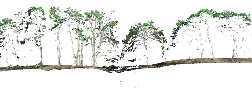
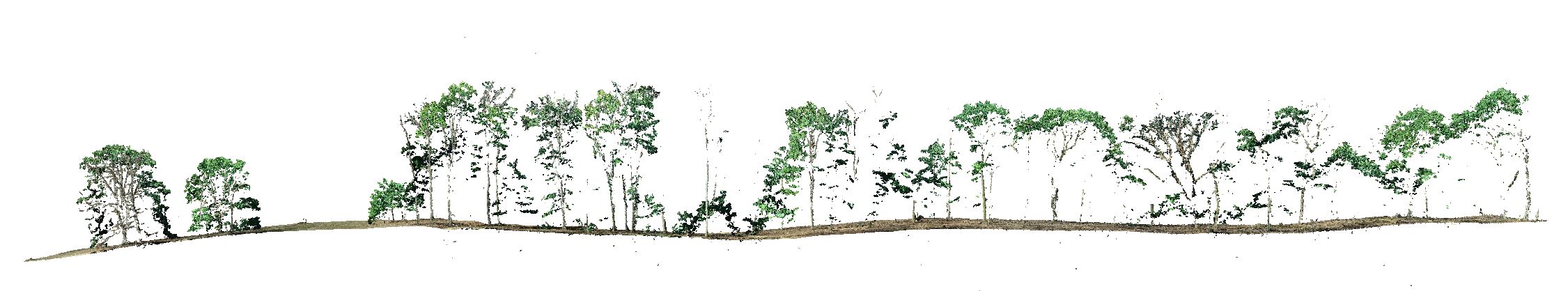
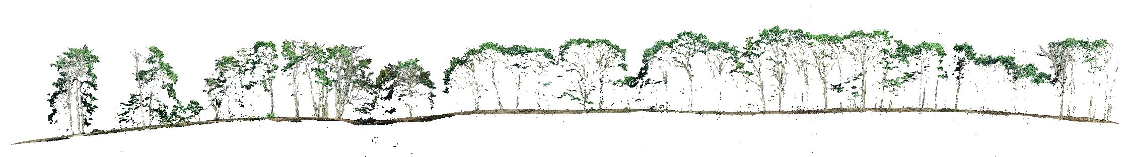
Leaf-Off mapping of deciduous forest structure holds some potential for the processing of terrain surface height under deciduous forests but with enough spatial resolution the resulting surface model also renders the leaf-off tree branch structure. Oblique 3D flight modi clearly have some potential here since the resulting point surface is very discontinuous and has a lot of depth. In the following figure a leaf-off model and the O4DGN point model was combined (extracted from a 16 m wide leaf-off transect). The resulting point cloud model clearly renders below canopy structure and as a combined data set this resembles Terrestrial Laser Scanning (TLS) point cloud data – although clearly lacking the various internal/horizontal leaf layers (the internal leaf structure is not detected in these combined point cloud models and the fused model is a multitemporal dataset from different dates – 15 months apart.

For this kind of analysis an airborne lidar & TLS dataset as a reference or accuracy benchmark dataset is clearly needed. We hope to have this sensor available by end of summer 22 but the equipment proposal is still in evaluation so lets keep fingers crossed.

This work was performed with Metashape 1.8.3 and Lastools (lastools academic license for FSU Jena – Institute of Geography). Flights were performed within the EDR-4 no-fly zone in Berlin with BLA permission for 2022 for the region Klein-Glienicke.

Update: overcast (NS and EW) transect point cloud numbers:

Flight plan type	No. of points in profile I (NS) Illumination: overcast (ground points)	No. of points in profile II (EW) Illumination: overcast (ground points)
N	770 754 (114 240)	1 004 728 (72 877)
DGN	1 275 930 (151 642)	1 584 001 (70 562)
O2	1 433 459 (117 120)	1 620 369 (72 146)
O4	1 987 933 (124 121)	2 433 253 (88 324)
O4N	2 168 572 (134 152)	2 592 288 (85 149)
O4DGN	2 253 685 (146 910)	2 746 086 (81 587)

All flight plans with overcast illumination conditions lead to higher point densities in the infinite voxel column statistics and in transect analysis (compare Tab. 2 and Tab. 4). However the complex oblique flight plans (O4DGN) generate comparable point numbers in this transect analysis for both overcast and direct illumination. For terrain ground detection already the simple Nadir flight plan with overcast illumination conditions provides better detection results than the direct sun light illumination version.

(Preliminary)conclusions: so yes it seems as if the O4DGN mode ends up with the highest number of points. It is however unclear in how far all these points add to the overall accuracy of the vegetation structure representation. The oblique modes clearly render more ground height (especially under crown structure edges facing south) and for terrain model interpolation these modes clearly are preferable and the oblique modes also render the sides of isolated crown objects or stand borders more accurately, this also applies to stand gaps – and in consequence this renders a more complete 3D surface representation of the forest surface (especially in stands with open stand surfaces. If we look into the profiles and compare sub canopy surface points there seems to be more penetration into deeper layers of the canopy volume. The differences will be measured by horizontal slicing the ground height normalized point cloud model. This can only be done with a smaller subset of the point cloud since the full point cloud size easily exceeds the TIN based approach in lasground_new -> tiles … . An illumination direction related effect can be seen at the tree crown edges with the image plans that were done with direct sun illumination. Overcast conditions do not create this effect. The oblique flight modi generate more points at the south facing crown slopes. The overcast illumination conditions render more details of the terrain surface even with very basic Nadir viewing flight plans (Table 4) compared to the direct sun illuminated imaging flight plans and this also applies to the complexer O4/DGN modes. However the point cloud increase is less pronounced. Preliminary terrain model analysis from all these flight modes clearly shows that terrain height visibility is greatly improved with oblique viewing angles. Best terrain height mapping approach is however with the leaf-off situation.

This work is presented in more detail as “live oral” at ForestSAT 2022 in Session PS 1 – SpS 03: Applications of drones in forestry: lessons learnt and way forward. Location: Lecture Hall 2.