Cluster & Batch Processing in Agisoft Metashape

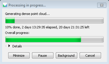
20 days! – better/faster hardware anyone?

Processing large quantities of image files from UAV flight campaigns in Agisoft is sometimes very time consuming and usually should be done in a  cluster environment with distributed nodes doing the heavy pixel lifting. Sometimes even a cluster setup can be limiting when the subprocess needs more RAM memory than available on a single cluster node. Together with the batch processing/scripting functionality of Agisoft this however shows great potential to also cope with bigger projects. There are also some tweaks that Agisoft published to increase processing speed that are not well known and seem to make a big difference (but might also compromise point cloud density).

Batch processing can be done in two different ways:

1. using the graphical batch processing tool in Agisoft Metashape or
2. using Python scripting language to trigger metashape-pro with the -r python-script.py option.

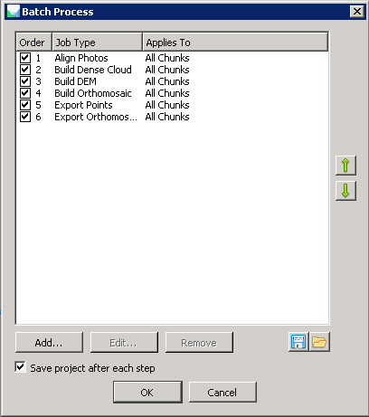
Using the batch processing tool is the easiest way to start working in a more automatic fashion with your files. Its invoked by opening “Workflow->Batch Process”:

Nearly all functions from the workflow section are available under “Batch Process”.  The Batch Process Manager also saves the project between different processes and can export results. The batch process itself can be saved as an xml file. Very handy for benchmarking tests.  This is likely what most people need but it still needs a graphical window  manager to be active.

Using a command line driven tool and batch scripting the automatic processing is much more flexible. Here Agisoft Metashape can also be utilized in an HPC environment.

A simple python script looks like the following snippet (opening a psx project, alignment, depth maps calculation and dense point cloud calculation:

import Metashape
Metshape.app.gpu_mask = 3
doc = Metashape.app.document
doc.open("photoscan.psx")
chunk = doc.chunk
chunk.matchPhotos(accuracy=Metashape.HighAccuracy, generic_preselection=True, reference_preselection=False)
chunk.alignCameras()
chunk.buildDepthMaps(quality=Metashape.HighQuality, filter=Metashape.MildFiltering)
chunk.buildDenseCloud()
doc.save()

Make sure that the GPUs are addressed correctly: 

The  GPU Mask needs to be defined. Confusing thing: the GPU mask is a binary number (integer) that defines which GPU to use. Using two out of three  GPUs  the binary is 110 (yes, yes, no). Two GPUs out of two would be 11. That binary is than converted to the decimal equivalent and defined under Metshape.app.gpu_mask = <mask>.

Masks:
enable 1 GPU = 1
enable 2 GPUs = 3
enable 3 GPUs = 7
enable 4 GPUs = 15

Cluster based processing:

The full power of the Agisoft Metashape software environment is however only unleashed with the distributed cluster based processing capabilities.
Agisoft differentiates into a coordinating „server“, the processing nodes and the clients. The client starts the processing by triggering a network based project batch job on the process coordination server, the process coordination is done by a dedicated server that queues the various jobs and starts the jobs on the processing nodes.
The client sends the project batch -> coordination server queues the different sub-processes and sends these to the nodes -> nodes process the sub-processes and report back when finished to receive the next process. If a node fails or is shutdown the job is canceled and will be send to a different node automatically. If all nodes are shutdown the coordination server will wait until a new node registers and will give this node the next job. A high number of nodes is not necessarily improving the overall processing speed because Agisoft cannot subdivide the project into tiny subprocesses – to work with very small sub-processes the project needs to have lots of smaller chunks pre-defined.

All nodes need to have rw access to the project data directory provided on a shared network drive. The access speed to the network drive seems to be critical for the overall speed. Especially the non-GPU  based processing is easily limited by the network speed of the cluster.

In order to use the cluster based node processing Agisoft Metashape Pro is started as a node instance from the command line:
/usr/local/metashape-pro/metashape.sh —node —dispatch XXX.XX.XXX.XX —root /archive2/data

The server instance is started on the server machine:
/usr/local/metashape-pro/metashape.sh —server —control XXX.XX.XXX.XX —dispatch XXX.XX.XXX.XX

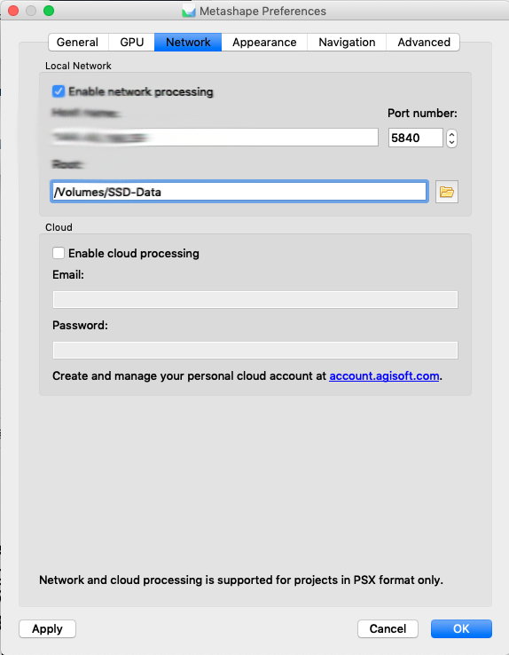
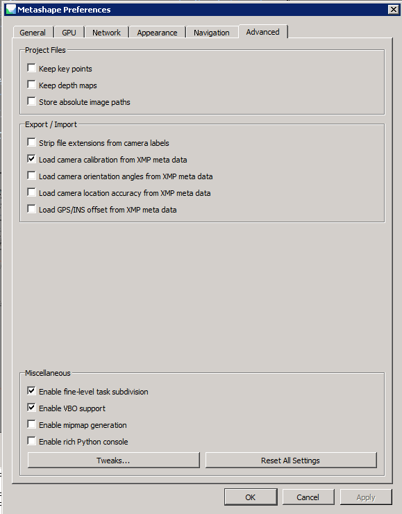
On the client machine Metashape-Pro network capabilities are configured in the preferences section. You select the dispatch server. Make sure that you have selected „fine level task sub division“ in the advanced section!

Starting a batch- job will than directly give you the option to process on the nodes. Very handy!

The Setup is as usual complicated by the read/write access to the shared network drive. It gets pretty complex when you combine Linux and Windows systems because the nodes all need to be linked to the right directory of the mount-point but its possible and useful.  The -root option does this and links to the right directory. In a heterogenous setup you can also define a specific machine as a GPU-only processor node. This is handy when one machine has strong GPUs installed.

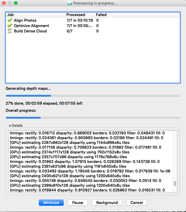
The cluster processing can be monitored with the network monitor:

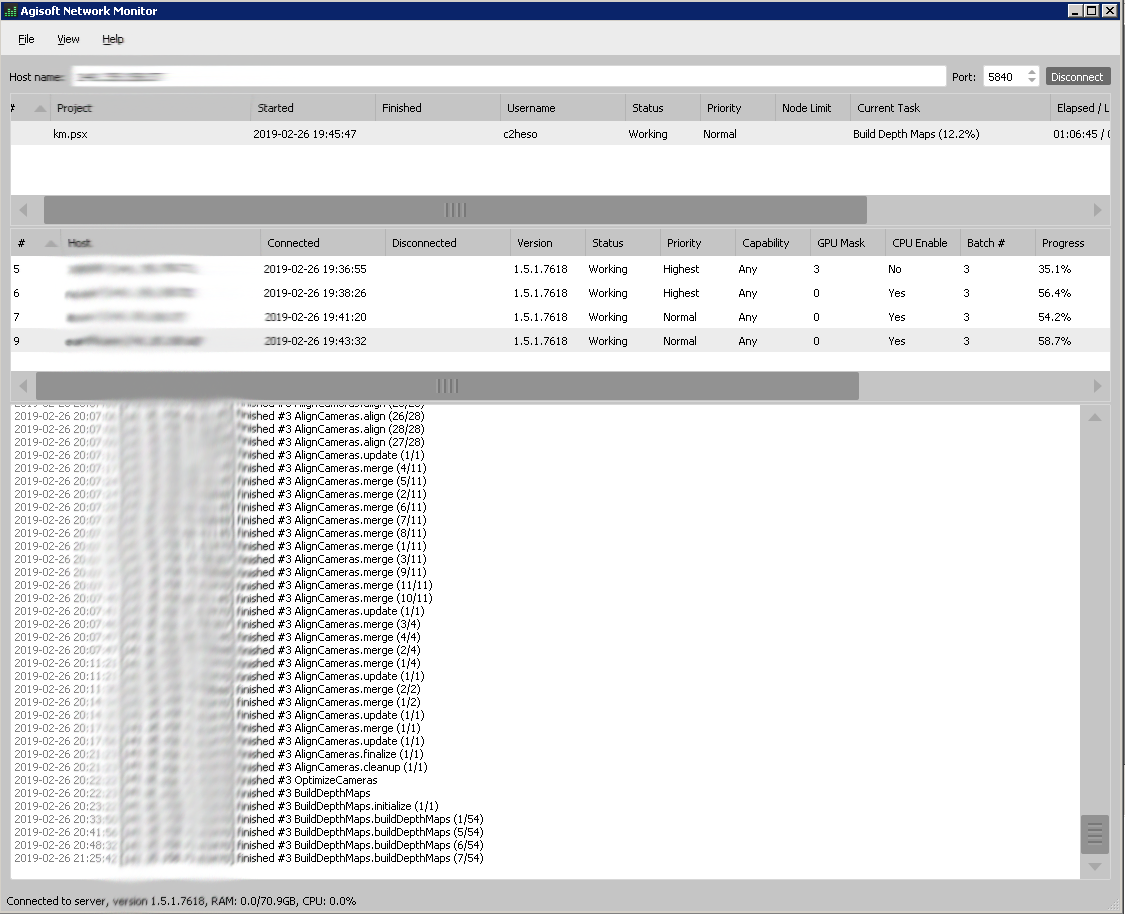
You can also easily change priorities in different nodes and setup some advanced GPU options here. But renicing the nodes seems to work more reliable in a Linux environment. Another nice detail: if one of your nodes is offline or fails for some reason, you can easily restart that node and add it to the server again. The configuration will be updated and the new node will be integrated into your working environment again (Agisoft states in the documentation that this can corrupt you project but I never experienced a problem that could be clearly linked to a offline node). Overall this is working nicely and seems to speed up bigger psx projects considerably  (doesnt work for psz projects), but speed improvements need at least 4 nodes to become interesting. It seems as if there is a strong drawback of processing of the network on a share directory so fast NFS or direct connections are better. Also SSD hard discs have an advantage here imo (see figure below).

Performance Boost and Benchmarking: 

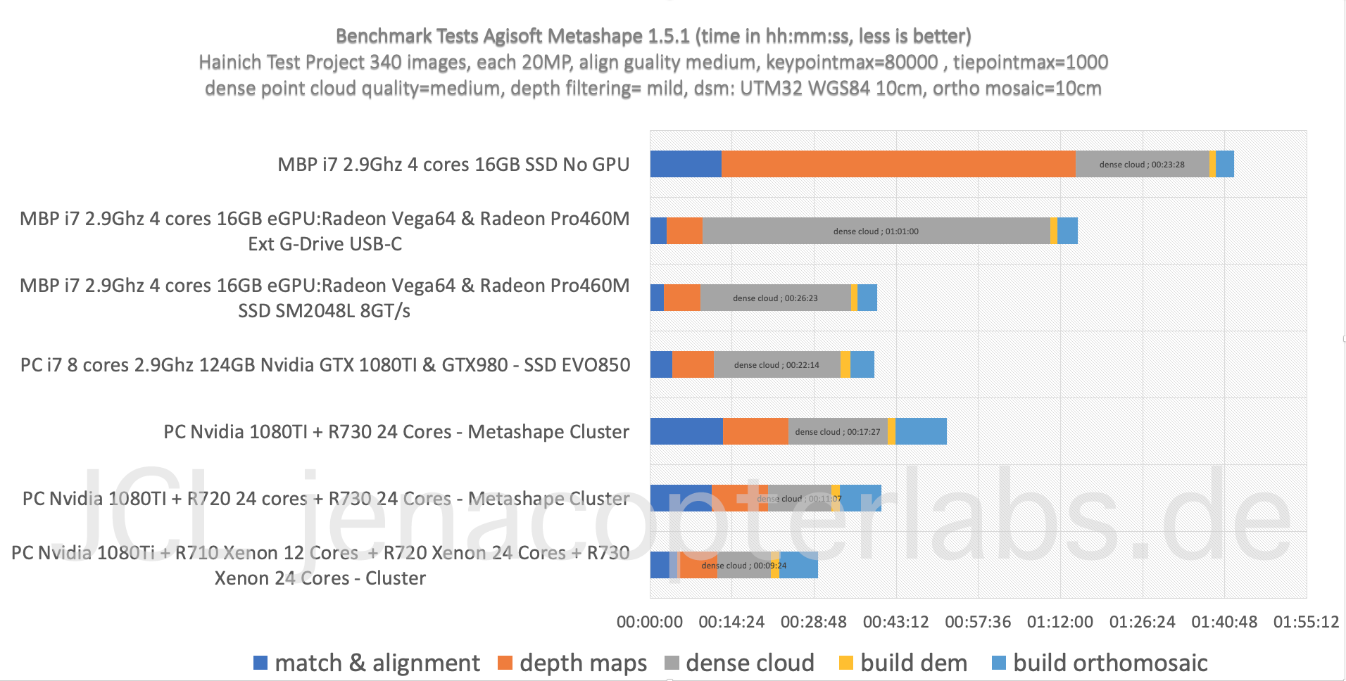
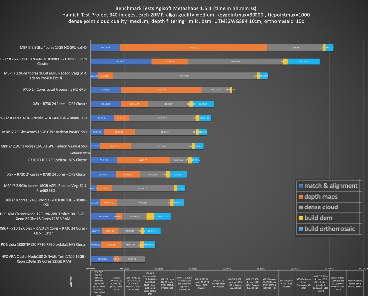
The following simple project from the Hainich NP project with 314 images (align quality=high, dense cloud quality=medium, point filtering=mild), was run in different configurations in a cluster setup:

1. Single MacBook Pro fully specified with eGPU Radeon Vega64 and Radeon Pro460M 16GB RAM on SSD
2. Single highend PC with 2 Nvidia GPU units (1x GTX1080Ti + 1x GTX980) 124GB RAM on SSD
3. highend PC with 2 Nvidia GPU units  + 1x Dell R720 with  24 Xeon cores and 124GB RAM
4. highend PC with 2 Nvidia GPU units  + 1x Dell R720 with  24 Xeon cores and 124GB RAM + 1x Dell R730 with 24 Xeon cores and 144GB RAM
5. highend PC with 2 Nvidia GPU units + 1x Dell R720 with  24 Xeon cores and 144GB RAM +1x Dell R730 with 24 Xeon cores and 124GB RAM + +1x Dell R710 with 12 Xeon cores and 72GB RAM
6. HPC ARA Cluster 5 Xeon Nodes (ongoing)
7. HPC ARA Cluster 19 Xeon Nodes (ongoing)
8. HPC ARA Cluster 52 Xeon Nodes (ongoing)
9. HPC ARA Cluster 4 Xeon Nodes 2 Tesla P100 16GB  (ongoing)
10. HPC ARA Cluster 1 Xeon Node 2 Tesla V100 16GB  (ongoing)

For this test run a typical full processing situation was batch programmed with initial alignment, dense point calculation, digital surface model calculation, ortho mosaic calculation. For accurate georeferencing you will also want to include GCPs from ground measurements with a DGPS. This step needs to be included before calculation of the georeferenced products (after alignment). If you are using a RTK UAV version than this is likely not necessary but good for validation.

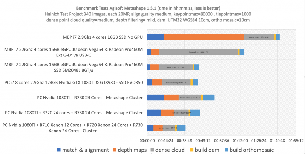
Since the mixed Dell Poweredge machines are not really comparable and the Dell R720/730/710 lack the GPU processing support from a dedicated GPU card, its obvious that the Nvidia GTX1080TI PC is likely doing the heavy image matching part (initial matching, alignment and depth map  calculations) but it is difficult to monitor if this is indeed the case or if other nodes also receive a sub task for these calculations. Clearly with this setup its also difficult to evaluate the saturation effect of adding more and more nodes to a cluster based processing environment, but even under these conditions the three R720/10/30 machines shorten the processing time to approx. 50% for the “dense point cloud” processing compared to local processing on an Nvidia PC. However compared to processing the same project on a eGPU AMD Radeon Vega64 based MBP (MacBook Pro) the initial matching and image alignment was slower on the cluster! This is likely due to the very fast solid state drive of the MBP but the VEGA64 GPU also seems to perform nicely here (a side note: the MacBook Pro would not allow very detailed processing setups due to the low RAM configuration, keypointmax and tiepointmax as well as dpc-quality was setup low for this test).  The network speed seems to limit the cluster. Next will be an extension of the benchmarking with the ARA FSU Jena HPC cluster (right now processing) with up to 300 nodes and two dual TESLA P100/V100 GPU cards.

Some preliminary findings:

1. GPU hardware accelerates initial matching and alignment and depth map calculation (as stated by Agisoft) but will not improve dense point cloud calculation time or DSM/Ortho mosaic processing (some sources online got this wrong).
2. Fast hard discs are clearly improving the speed for the “dense point cloud” task. The very fast SSD in a fully specified MacBook Pro with eGPU performed surprisingly good compared to the cluster configuration (but see “Side Note” comment).
3. Cluster based processing is somehow limited by the network drive speed/rw access speed. The clustering however clearly improves processing speed especially for the “build dense cloud point” task and this is the most time consuming part of the workflow and takes usually days in the full resolution image mode (“ultrahigh” setting). Thats why even smaller speed improvements are very relevant. However since the slowest node can become kind of a bottleneck for the full processing time – its important to have equally specified nodes in the cluster. In our cluster we combined 3 different Dell Poweredge systems with a PC. Faster network drive configuration will clearly improve the processing time (NFS!).

Some prerequisites for cluster processing:

• all nodes need the exact same version of the Metashape-Pro installation,
• you will need at least 3 Agisoft Metashape Pro licenses to get some speed benefit when you work in a slow network configuration!
• all nodes must have rw access to the project directory over a shared fast network drive,
• ultrahigh dense point cloud settings with thousands of images clearly depend on the RAM hardware specs. RAM needs can easily exceed the available capacity and the CPUs will just stop processing anything. A solution is to work with more and smaller sub chunks within a project – reducing the size of the subprocess memory consumption and needs. As a consequence point clouds and ortho products needs to be merged later.

Tbc with the FSU Jena HPC ARA cluster and the TESLA V100/P100 cards. First results with the TESLA cards show promising results accelerating at least specific parts of the workflow!

Find more related infos in the Agisoft forum and the Metashape Python reference manual .

Update: HPC Processing on TESLA GPUs

Results from testing with the TESLA V100 GPUs are available here and within the PDF of my presentation for the Research Colloq held in summer 2019. Feel free to download the PDF file of this presentation here: PDF Link

Overall the TESLA GPUs clearly performed very well on the “Depth Map” calculations. Here processing time was only approx 1/3 of the VEGA64 processing times. However the TESLA GPUs did not help much with the calculation intensive “Dense Cloud” process since here most of the work is done on CPUs. The results with the two TESLA V100 cards was kind of disappointing since these cards are so expensive. However the TESLA GPUs are likely better suited for Machine Learning tasks / CNN classifications and the like and might not perform as good with Agisoft.

The HPC environment of the FSU Jena (Ara Cluster) can be used in configurations with multiple CPU nodes (overall 300 compute node with each 12 cores) but we did not finalized test these configurations with Agisoft since the SLURM front end never allowed to process on these partitions in a priority mode. So one hardly knows if the partition is yours right now or if some molecular modeling is doing heavy number crunching at the same time.  

So far it seems as if configuring a speedy setup with multiple Gaming GPUs and a very fast and big SSD is the way to go. For the “dense point cloud” processing sub task multiple CPUs on a Dual or Quad CPU socket board or combining multiple machines with with very fast connections (TB3) would be useful. Very big processing projects (more than 300 images with each 20MP) clearly need a good RAM setup with more than 128GB RAM.