AMAPVox for Metal GPU Power: Claudes redesign for the Mac

Ok – take a breath! This is about Anthropic Claude and since everyone uses one of the LLM approaches for coding it’s time to name it.  I had some hope regarding metal (Mac) processing power for large volumes of LiDAR points but ultimately you always have to face some restrictions when you work with packages that were designed for other (or all) hardware architectures. Not so anymore with Anthropics Claude Code engine. AMAPVox is an open-source LiDAR point cloud voxelization software and companion R package used in forestry and ecology to analyze 3D vegetation structure. It tracks individual laser pulses through a 3D grid (a voxelized space) and calculates local transmittance/attenuation per voxel. It estimates leaf area density (LAD) and plant area index (PAI) using various theoretical and numerical approaches. Thats why its an important tool for derived LAI measurements directly from Leaf-Off/On LiDAR data. But AMAPVox is comparably slow as a Java design on Mac – so I let Claude fully redesign AMAPVox (Vincent et al. 2017, Pimont et al. 2018) for the Metal shader architecture from Apple from scratch (but without TLS-formats, GUI and without the Viewer). This took just two hours including testing. Comparisons with the original CPU-based AMAPVox on Java compute 99.999% of the same values. A simple switch in my processing pipeline now just changes to “MVox” and the full ray tracing is accelerated by factor of 4-5 at least. So for the 3 billion (Mrd. in German) points of the winter- and summer-point cloud of “Neuer Garten” park region MVox now needs just 20% of the time AMAPVox needed.

Some functional difference: MVox also calculates a clumping index, and simulates a cone ring with 7 or 19 (2 rings) multiple beams (instead of one beam), This is much closer to the real world situation since the beam widens at the end and the diameter can cover more that one voxel. The beam number is split as a consequence of this approach over multiple voxels when the cone multi-beam shot covers multiple voxels. Neighboring voxels receive only a fraction of the original beam number but the result is overall more accurate (this mainly applies to small voxel size setups / or larger beam sizes and the –core 19 option increases processing time considerably, for L2 data from 110m altitude and 0.5 m voxels the difference is more of academic nature but it can be measured). MVox reads the same xml config, and writes the same .vox file or NetCDF and uses the same compute code from CeCILL-B-Source but it’s not a copy of the source code. For calculation of corrected PAD values the R AMAPVox library is loaded again.

I wonder what all this means for software coding in general. Right now with Claude Code Fable 5.1 or Opus 5.5 (autumn 2026) you can easily optimize and recode every open source package there is (if license permits it)..

What MVox does different than AMAPVox (apart from some functional differences – see above):

MVox is faster mainly because of how it organizes data. The GPU’s raw speed is a smaller portion of it. In order of impact:

1. One thread instead of thousands. AMAPVox’s ray-tracing loop processes one pulse after another. Its thread pool is sized to the number of scans. With a single scan it runs in the calling thread, so the threads-per-task option has no effect in the pipeline. A second thread builds the pulses and passes them on through a blocking queue, and the method that builds them is itself synchronized. The pipeline got its parallelism only by running two configurations per block in three to five queues. In the first test runs three queues used less than half of the 16 cores. MVox runs one GPU thread per pulse and spreads reading, pulse building and writing over all CPU cores.
2. Far less work per voxel crossing. In the bytecode, every crossing creates a new list and free-path objects. At each step the voxel walker creates a crossing context, an index object and several vectors. The test whether the next echo lies in the current voxel creates a point, an index and a boolean array. The beam cross-section creates another point. With the PPL estimator on, each hit also creates a lambda and a record object. Every voxel update takes a lock, and PPL adds a second one. Each pulse is walked twice: once to the ground for the potential beam surface and once for the propagation. The JIT can remove some of these allocations, but not the objects that are stored in lists. MVox walks each pulse once for both purposes and allocates nothing in the kernel. Each step recomputes the boundary distances from integer indices with a few multiply-adds. About a dozen atomic additions per crossing are now its main cost.
3. Flat data instead of objects for every pulse and echo. AMAPVox has eight allocation sites in its pulse-building code. Each echo gets a line segment, a point, and an echo object with two hash maps that hold boxed attribute values. MVox stores pulses and echoes in flat arrays of 36 and 16 bytes per entry. It computes each echo’s voxel, weight and filter flag once, in a parallel CPU pass, so the kernel only compares three integers.
4. Estimators. AMAPVox’s post-processing is a single-threaded loop over all voxels. Its PPL search evaluates a Java stream over each voxel’s records up to 200 times. It keeps a transmittance record object for every crossing, which caused the earlier out-of-memory failures. PPL records exist only for hits. MVox stores records as 16-byte structs in slabs and runs the search on the GPU.
5. Reading and output. AMAPVox creates one object per point and checks echo consistency with several Java stream pipelines per pulse. It writes the voxel file in one thread and looks up every field by name through reflection for each value. MVox memory-maps the file and decodes it in 64 parallel chunks. It sorts with a radix sort and writes the x-slices in parallel with its own number formatter.
6. Single precision in the kernel. The kernel computes in 32-bit floats, which halves memory traffic. Double precision is kept where it matters, for building pulses and assigning echoes to voxels.

Some comparisons from the pipeline:

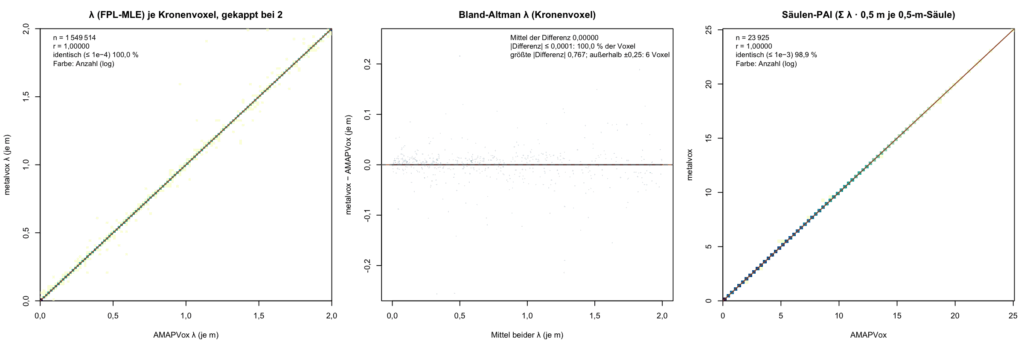
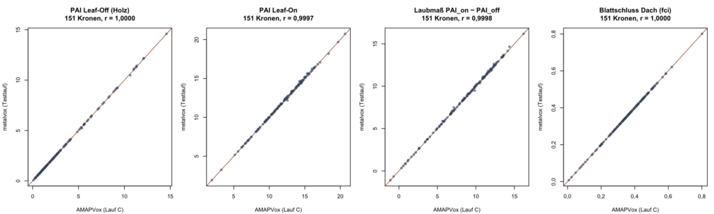
Fig. 1: Comparison of AMAPVox versus MVox results, PAI Leaf-Off/On, PAI-Diff, fci, FPL-MLE and PAI for 0.5m voxel columns. Results are basically identical.

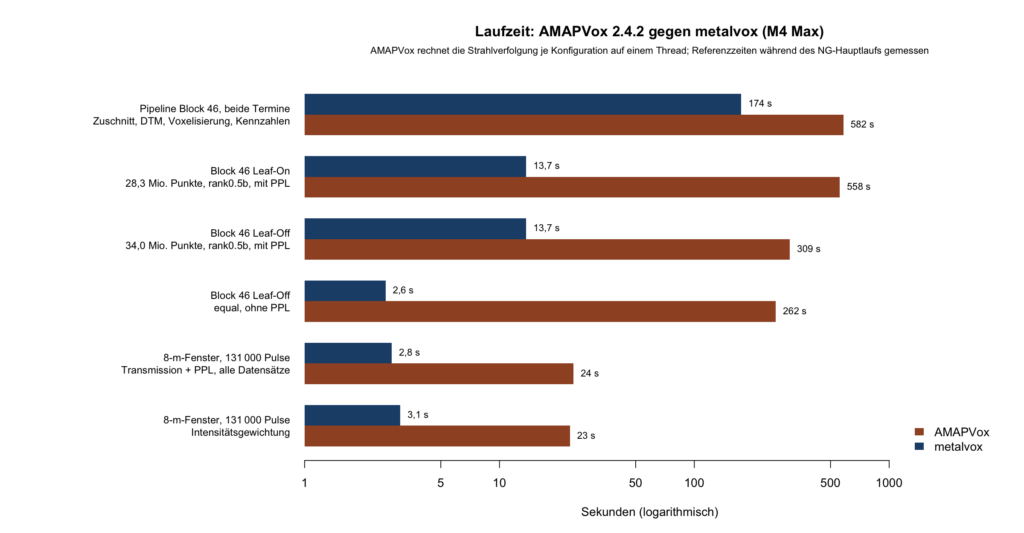Fig. 2: Speed difference AMAPVox 2.4.2 versus MVox based on LiDAR point cloud Leaf-On/Off data from Park3D, x in log scaled.

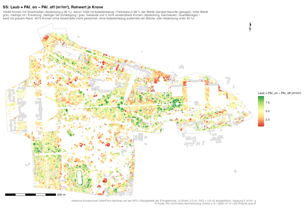
Fig. 3: Per tree crown species specific LAI measurements for the Sanssouci Park area based on LiDAR PAI Leaf-Off and Leaf-On difference calculation. Calculation based on MVox an AMAPVox compatible (Vincent et al. 2017, Pimont et al. 2018).